
INTRODUCTION
In the medical field, disabilities are symptoms that make it difficult for an individual to perform daily tasks. Various types of brain traumas and illnesses can cause dementia. The most prevalent kind of dementia is Alzheimer’s disease (AD), accounting for 60-70% of cases. Dementia is a significant factor that contributes to disability and dependency among the elderly population. Individuals with AD will eventually experience severe symptoms that can make the condition a disability. AD causes cognitive impairment, amnesia, and a loss of brain functions and independence ( Ulep et al., 2018). AD is a global health concern that affects many people and their families. It also puts a significant financial burden on healthcare systems around the world. It is estimated that by 2050, around 152 million people worldwide will be affected by AD, up from the current estimate of 47 million ( Patterson, 2018). The precise mechanisms behind the development of AD have not been fully understood, and currently, there is no medication that can completely cure or stop the progression of the disease.
Screening people with mild cognitive impairment (MCI) to detect AD early is essential. This can help in providing better care and management, as well as developing new drugs and preventive measures that can slow down the progression of the disease. Brain magnetic resonance imaging (MRI) can be used to examine changes in the brain that are associated with AD without the need for invasive methods.
The early and accurate detection of AD is crucial to minimize its significant impact on patients and society. Identifying AD in its early stages is crucial due to its cognitive impairment manifestation. The progress in AI and medical imaging has opened new avenues for early-stage AD prediction, enabling timely and effective treatment.
The widespread adoption of digital technology in healthcare has resulted in healthcare providers generating vast amounts of multimedia medical data. Integrating artificial intelligence (AI) into healthcare has led to its application in smart healthcare systems, patient care, and diagnostic improvements. AI has enabled the achievement of goals that were previously unattainable in the healthcare sector ( Yang et al., 2016; Gadekallu et al., 2020).
AI-powered deep learning (DL) techniques can efficiently evaluate large medical data with high precision. DL has the potential to effectively analyze large quantities of diverse medical data, empowering clinicians to more accurately diagnose diseases and predict their outcomes.
Various studies ( Hossain et al., 2019a, b) have demonstrated that using DL and convolutional neural networks (CNNs) to develop disease prediction models has resulted in significant progress. Therefore, implementing DL techniques in the field of disease diagnosis is currently regarded as a dominant trend. There are different methods used to diagnose AD, such as clinical assessments, cognitive assessments, and various imaging techniques. However, these methods often fail to identify the disease in its early stages, when it is easier to manage. Therefore, it is vital to focus on timely and accurate detection of Alzheimer’s. AI can be a game changer in Alzheimer’s research and patient care. It holds great potential for significant progress in this field.
Dementia is a term used to describe cognitive decline in AD and other neurological conditions. Alzheimer’s has three stages: mild, moderate, and severe. In the early stage, individuals may have MCI, but they can still function independently. However, they may experience difficulty recalling words or item locations. Medical professionals can diagnose these symptoms using specific diagnostic tools. It is essential to seek diagnosis and treatment promptly to manage the symptoms and improve the quality of life.
The intermediate stage of AD, commonly referred to as moderate AD, is a phase that is often prolonged, spanning several years. As the disease progresses, those diagnosed with Alzheimer’s require an increased level of caregiving. During this stage, the symptoms of dementia become more manifest. Individuals experiencing cognitive impairment may exhibit symptoms such as confusion with words, emotional frustration, and unpredictable behavior, including resistance to personal hygiene activities. This stage may also result in challenges for individuals in articulating cognitive processes and executing mundane activities independently due to the impairment of neuronal cells within the cerebral region.
In the advanced phase, AD becomes severe and is characterized by the manifestation of severe symptoms of dementia. This phase is commonly referred to as severe Alzheimer’s. As the condition progresses, individuals experience a decline in their ability to effectively engage with their surroundings, engage in meaningful discourse, and regulate their physical mobility. Although individuals may continue articulating words or sentences, expressing their feelings and emotions becomes increasingly difficult. As memory and cognitive abilities decline, notable changes in personality may occur, requiring comprehensive caregiving for affected individuals ( Alzheimer’s Association, 2023).
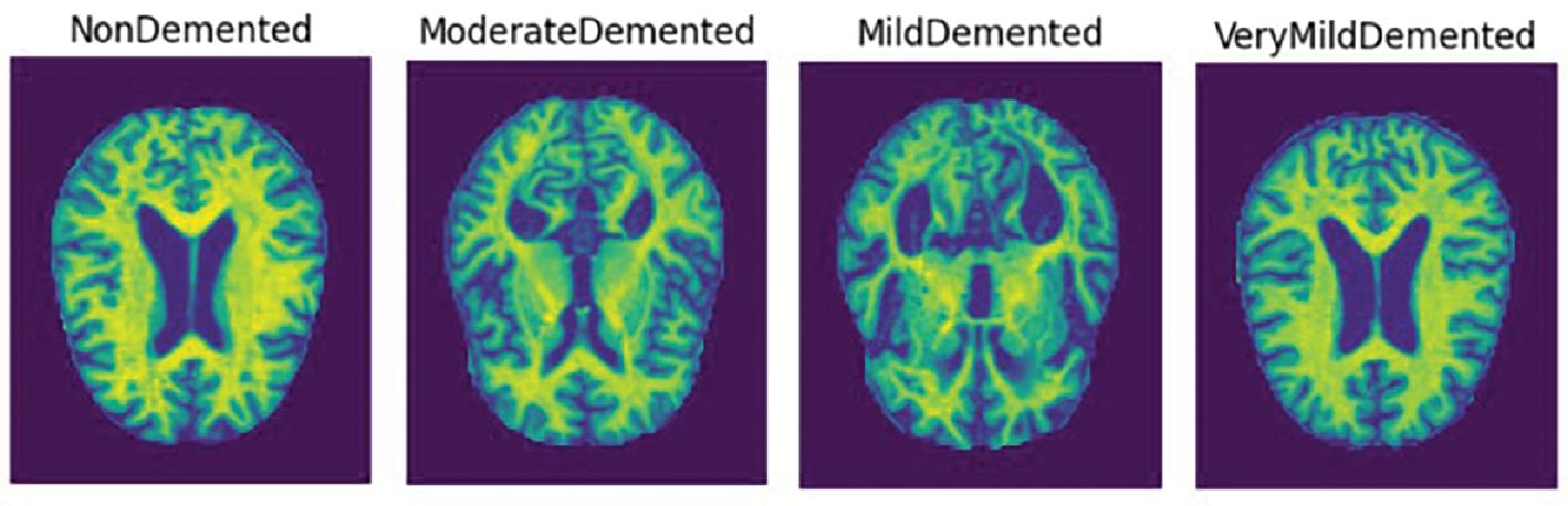
There are four classes of Alzheimer’s dementia: mild, moderate, non-demented, and very mild. Figure 1 shows examples of each class.
An automated diagnostic system is necessary to aid healthcare providers in detecting Alzheimer’s dementia at its early stages. The use of machine learning techniques has shown significant progress in illness diagnosis applications compared to conventional computer-aided diagnosis systems. Manual procedures are required to extract features in machine learning techniques, which can be challenging and require specialized knowledge from ophthalmologists in the specific sector.
DL models can automatically extract features, reducing the need for extensive data engineering. Many DL models have been proposed for analyzing MRI images to identify Alzheimer’s dementia.
CNN models are commonly used for medical image analysis and disease diagnosis ( Lecun et al., 1998; Yann et al., 2015). CNN models were first used in the ImageNet competition in 2015 and are now commonly used in image processing research, including feature extraction, object detection, and natural language processing.
The following are the research’s contributions:
In this study, MRI images were used to classify Alzheimer’s dementia using a CNN model. A weighted loss function was used to address data distribution imbalance and improve the model’s performance. Its outcomes were compared with three pre-trained models to showcase its effectiveness.
The following sections of the article are organized as follows: in the Related Works section, we analyze and examine prior works that are relevant to the topic being discussed. The Materials and Methods section outlines the materials and methodology used in this study. This section primarily focuses on the technique of data pre-processing and the approach to addressing the issue of dataset imbalance. In the Proposed Model section, we discuss the proposed model and its performance and compare the findings with those of the pre-existing models. Finally, the paper concludes in the Conclusion section.
RELATED WORKS
This section provides an overview of methodologies and their contributions, analyzing studies in AD prediction through AI approaches.
In the beginning, attempts to predict AD mainly used traditional statistical methods. One study conducted by Bertram et al. (2010) used genetic data to identify several genes that are linked to increased risk. However, these methods lacked the necessary level of accuracy required for clinical diagnosis.
Mateos-Pérez et al. (2018) reported the use of MRI in machine learning to predict AD. Various methods were employed, including random forests ( Tripoliti et al., 2011), support vector machines (SVMs) ( Van Leemput et al., 1999), and boosting techniques ( Hinrichs et al., 2009).
Ghazal and Issa (2022) have introduced a transfer learning-based model that performs multi-class classification on brain MRIs. This model can classify the images into four distinct categories, namely mild dementia, very mild dementia, moderate dementia, and non-dementia. The accuracy of the proposed model is 91.70%.
Kavitha et al. (2022) developed a model to predict AD. SVM, gradient boosting, decision tree, and voting classifiers are employed to detect AD. The accuracy of the proposed model is 83%.
Uddin et al. (2023) proposed a model that uses multiple classifiers to identify AD. The model achieved an accuracy of 96% with the voting classifier. The authors concluded that machine learning can help reduce mortality rates by accurately identifying AD.
Eskildsen et al. (2013) were able to enhance the accuracy of medical diagnoses by utilizing machine learning techniques on brain imaging data. Studies conducted by Liu et al. (2014) and Arbabshirani et al. (2017) have further expanded the application of machine learning techniques to include neuropsychological and clinical data, which has made them more effective at predicting outcomes.
CNNs have shown promise in predicting Alzheimer’s based on MRI data. Liu et al. (2020) used CNNs for feature extraction, resulting in high accuracy and interpretability.
Martínez-Murcia et al. (2020) used deep convolutional autoencoders to analyze AD data and performed regression and classification analysis to determine the impact of each coordinate of the autoencoder manifold on the brain. They achieved over 80% prediction accuracy when diagnosing AD.
Prajapati et al. (2021) created a deep neural network for binary classification with distinct activation functions. The k-fold validation process selects the best-performing model. A Lancet Commission study states that 35% of AD risk factors are modifiable.
Helaly et al. (2022) developed a CNN model to diagnose early-stage AD. It uses two methods for AD prediction. A web app enables remote screening of AD and identifies the AD stage. The VGG19 model identifies AD stages with 97% accuracy.
Khan et al. (2021) proposed a technique for diagnosing AD using MRI images. The method achieves an accuracy rate of 93% by combining deep learning algorithms with image processing techniques. Additionally, the approach attains a BAC of 0.88 in identifying the disease stage and distinguishing between very mild, severe, and healthy tissue phases of the disease.
Rao et al. (2023) proposed a technique that combines multi-layer perceptron (MLP) and SVM methods for predicting and classifying AD by analyzing MRI images. The technique involves converting three-dimensional images into two-dimensional (2D) slices for the purpose of feature extraction using MLP, followed by the application of SVM as a classifier.
In the study by Venkatasubramanian et al. (2023), the researchers utilized MRI data to create a DL framework that is capable of classifying AD and segmenting the hippocampus simultaneously using multi-task DL. The capsule network CNN model was optimized with the deer hunting optimization method for the purpose of sickness classification. To test the effectiveness of the proposed technique, standardized MRI datasets from ADNI were used for evaluation. Table 1 summarizes the models and their accuracy for Alzheimer’s disease classification.
A related work summary of Alzheimer’s disease classification.
| Research | Models applied | Accuracy (%) |
|---|---|---|
| Martínez-Murcia et al. (2020) | DL | 80 |
| Liu et al. (2020) | CNN | 88.9 |
| Prajapati et al. (2021) | Transfer learning | 85 |
| Khan et al. (2021) | ML and DL | 93 |
| Uddin et al. (2023) | ML | 96 |
| Helaly et al. (2022) | CNN | 97 |
| Ghazal and Issa (2022) | Transfer learning | 91.7 |
| Kavitha et al. (2022) | ML | 83 |
Abbreviations: CNN, convolutional neural network; DL, deep learning; ML, machine learning.
MATERIALS AND METHODS
This study analyzes a public MRI dataset ( Kaggle, 2020) that includes 5121 training and 1279 testing images. The dataset comprises four classes: “MildDemented,” “ModerateDemented,” “NonDemented,” and “VeryMildDemented.” All the images have the same shape: (208, 76, 3). Each image is colored and has the dimension: width = 208, height = 76.
Image pre-processing
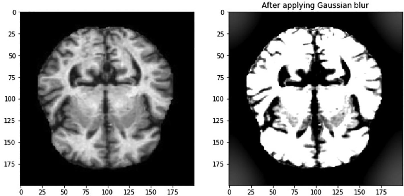
Gaussian blurring is a widely used technique in image processing that helps in reducing the noise present in images. Even though fine features may be lost, Gaussian blurring reduces image noise while maintaining low spatial frequency components, similar to a non-uniform low-pass filter. The process of Gaussian blurring an image involves the use of a Gaussian kernel. The formulation of the 2D Gaussian kernel is as follows:
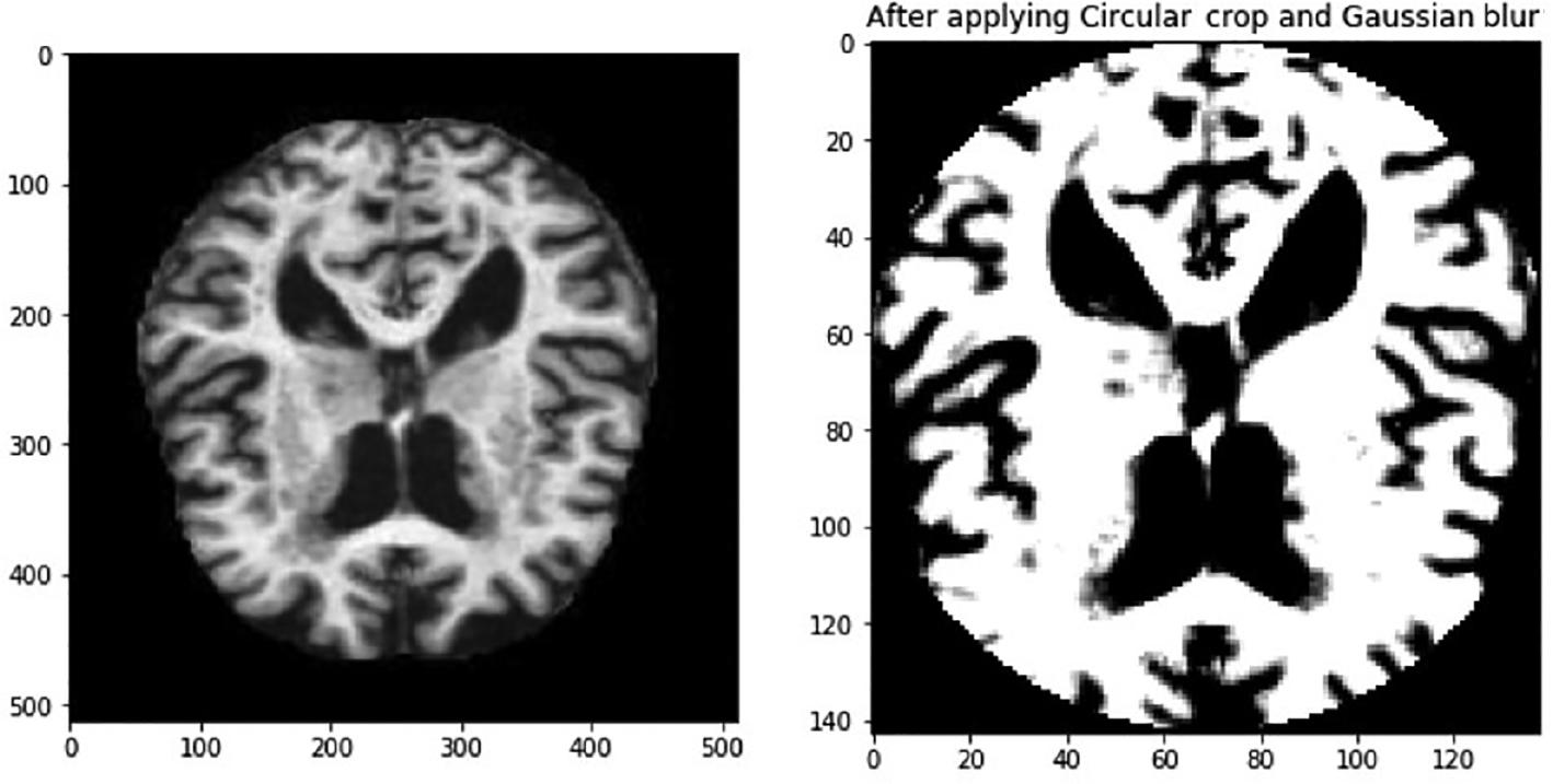
In this context, σ symbolizes the distribution’s standard deviation, whereas x and y are used to denote the respective locations of the index. The parameter σ is used to measure the amount of variation around the mean value in a Gaussian distribution. This method is used to determine the level of blurring around a pixel. The Gaussian blurring technique improves the visibility of feature details, and this is demonstrated in Figure 2. The features within the eye are now more visible. In addition, the images show that there are black areas in some images that do not provide any useful information. It is important to take this into account when we reduce the size of the image, as the areas that contain important information may become too small. Therefore, it is necessary to crop the image to eliminate the uninformative regions. The image in Figure 3 is an example of circular cropping and Gaussian blurring techniques applied to an image. It is recommended to convert images to grayscale to visualize them accurately due to the variability of lighting conditions and the challenges they pose for perception. An alternative strategy called the Ben Graham method is known to be more effective. Ben Graham presented it as an innovative approach to improving lighting conditions and enhancing accuracy. Therefore, this study aims to examine this methodology. Using Ben Graham’s methodology, several significant intricacies in the eyes can be uncovered.
Imbalanced data handling
Analyzing large datasets requires exploring the class distribution and correlations in dispersed data with significant dimensions. Performing certain tasks manually can be extremely difficult and sometimes impossible. In such scenarios, the t-distributed stochastic neighbor embedding (t-SNE) technique can be of great help. This technique reduces the number of dimensions in data ( van der Maaten and Hinton, 2008) and is usually employed to provide a visual representation of datasets that contain a large number of dimensions. t-SNE is a commonly used technique for visualizing the distribution of data points belonging to different classes in a dataset. This visual analysis is crucial for all machine learning systems. The t-SNE output in Figure 4 demonstrates how MRI image attributes can group patients with AD by severity. It is apparent that the classes “NonDemented” and “MildDemented” can be easily distinguished from the other classes. However, it is extremely challenging to differentiate between the other classes. Therefore, it is crucial to use an intelligent model to accurately categorize the severity classes of Alzheimer’s. We have just examined two principal component analysis (PCA) components while employing the PCA approach.
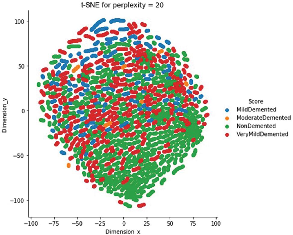
t-SNE visualization of the Alzheimer class clustering. Abbreviations: MRI, magnetic resonance imaging; t-SNE, t-distributed stochastic neighbor embedding.
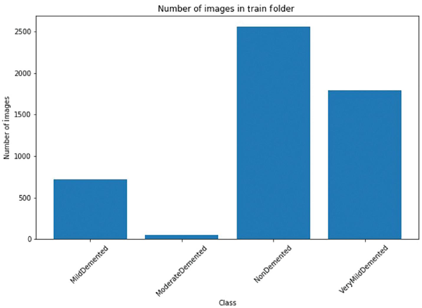
Data scientists often face several challenges in processing data before creating a machine learning model for a particular dataset. One of the issues they encounter is the presence of class imbalances in the data. Medical datasets, in particular, tend to have a significant disparity in class distribution. The MRI image dataset is no different. Figure 5 displays the frequency distribution of the classes. The result exhibits a significant variation in the prevalence of positive instances among the different Alzheimer classes. Regrettably, this disparity is present across the entire dataset. In order to avoid issues with data imbalance while training our model, we need to develop a quick training method. This can be achieved by using a dataset that has an equal representation of both positive and negative cases. By doing so, we can ensure that the loss is balanced for both types of cases during model training.
Class imbalance’s effects on the loss function
When a dataset has an imbalanced class distribution, it can pose a significant challenge for categorization tasks. A highly skewed dataset can result in suboptimal predictive accuracy for the minority class in a predictive model.
Data imbalance is a common issue in machine learning, but it can be addressed using different methods. One such method is data augmentation, which generates extra training data by transforming the current dataset. However, using data augmentation can increase the training duration for the model. It is typically employed when the model requires a large dataset for training, which may not be easily accessible ( Choi et al., 2017). In this research, we used a large MRI dataset and applied various data augmentation techniques to classify MRI images effectively.
Image classification can be very challenging when the classifier is trained using an unbalanced dataset. Conventional deep neural networks treat every individual sample equally and use the same level of penalization for the training loss. This becomes problematic when the training data have imbalanced classes, compromising the model’s ability to accurately represent the minority class. A non-uniform-weighted loss function is used in the suggested model to solve this problem. This loss function specifically accounts for the training loss bias toward the minority class, mitigating the issue. The following section explains the weighted loss function and strategies for correcting the imbalance in the minority class. Throughout the training process, the model is trained using this loss function.
For each image, conventional cross-entropy loss should be taken into account. Hence, the following expression can be used to indicate how the cross-entropy loss affects the ith data sample:
In machine learning, we use notations to represent different elements. For instance, we use x i to denote the input features, y i for the label, and f( x i ) to represent the likelihood that the model will produce a positive value. During the training process, y i can either be zero or (1− y i ) can be zero. This means that there is only one element that leads to the loss, whereas the other factor results in a value of zero. Therefore, the mean loss for the entire training dataset, which has a size of N, can be calculated as follows:
When a model is trained on a highly imbalanced dataset with relatively few positive classes, the usual loss function will be more affected by the negative class. To address this issue, we can calculate the total loss contribution of each class in the entire training dataset and then combine them. This allows us to express the contribution of each class more accurately.
and
The positive and negative frequencies for each Alzheimer class are shown in Figure 6. The figure also presents the contribution ratios side by side for each Alzheimer class.
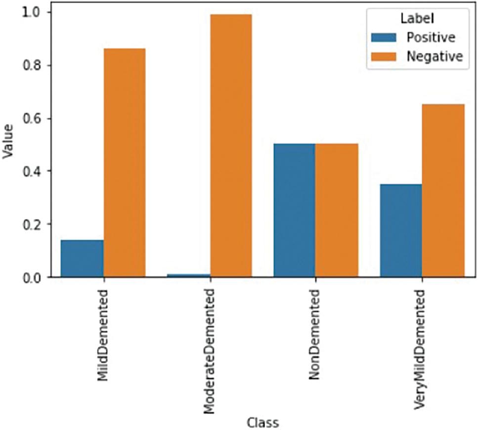
According to the graph, negative cases make a greater contribution than positive cases. However, it is important that both classes contribute comparably during the model’s training process. To achieve this balance, a weight factor specific to each class ( w pos and w neg ) is applied to every sample in each class. This ensures that each example contributes equally, as demonstrated below:
This may be accomplished easily by simply taking
During training, positive and negative situations are balanced. Figure 7 displays a well-proportioned case.
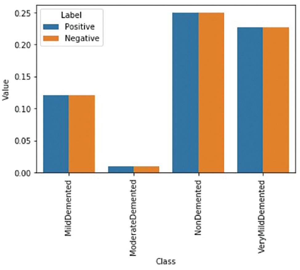
The image demonstrates that when these weightings are applied, both the positive and negative examples of each class will have an equal influence on the loss function. As a result, the computed weights are used to calculate the final weighted loss for every training example, which looks like this:
THE PROPOSED MODEL
This article presents a light-weight CNN model to identify AD from MRI images. The model is depicted in Figure 8. The model comprises four 2D convolutional layers, the first two of which have 32 filters and the subsequent two of which have 64 filters. The filter size is 3 × 3, with the same amount of padding in all layers, and the “ReLU” activation function is applied in every layer.
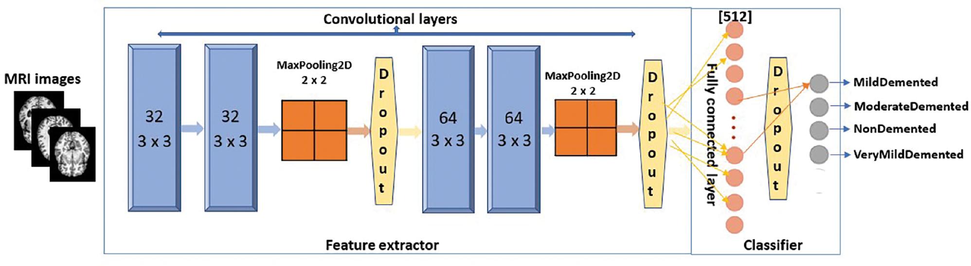
The proposed CNN model. Abbreviations: CNN, convolutional neural network; MRI, magnetic resonance imaging.
The model used in this study employs the MaxPooling2D layer after the second and fourth levels. Dropout regularization is integrated following the second, fourth, and fully connected layers. As it is a multi-level classification, the classification layer uses the Softmax activation function. The initial learning rate used in the model is 0.0001, with a decay value of 0.000001 and a minibatch size of 8 for both the training and validation phases. The model also uses a factor of 0.5 to modify the learning rate, following the formula lr = lr * factor.
The model employs the RMSprop optimizer ( Ruder, 2021). RMSprop helps to reduce oscillations and automatically adjusts the learning rate. This optimizer divides the learning rate by an exponentially decaying average of squared gradients. By doing so, RMSprop prevents excessive exploration along the path of oscillations. Additionally, it assigns a unique learning rate to each parameter. The equation below illustrates the update of the learning rate.
For each parameter w j
The symbol μ represents “initial learning.” The variable v t represents the exponential average of the squares of the gradients, and g t represents the gradient of w j at time t. Furthermore, the Adam optimizer combines the heuristics of RMSprop and momentum. The subsequent equation illustrates the computation.
For every parameter w j
Here are the symbols’ description: the symbol μ represents the initial learning, and v t represents the exponential average of gradients. w j and g t represent the gradient of w j at time t. The exponential average of the squares of the gradients along w j is denoted by s t . β 1 and β 2 are hyperparameters.
The Softmax activation function was used in the CNN model to generate the classification probability for each MRI image. This probability ranges from 0 to 1. The Softmax activation function is a commonly used classification layer in CNN models. It is typical practice to convert the output scores of the network into a normalized probability distribution. The following equation defines the Softmax function:
where denotes the input vector, z i represents the elements in , represents the exponential function, and denotes the normalization term.
The parameters used for training the proposed model are listed in Table 2.
Parameters for model training.
| Parameters | Value |
|---|---|
| Initial learning rate | 0.0001 |
| Decay rate | 0.0000001 |
| Batch size | 32 |
| Shuffling approach | Every epoch |
| Optimization function | RMSprop |
| Maximum epoch | 25 |
| The environment of execution | GPU |
Abbreviation: GPU, graphics processing unit.
Performance analysis
The dataset used for this study comprises 5121 images for training and 1279 images for testing. In addition, 80% of the training dataset is used for model training, and the remaining 20% is kept aside for validation. Figure 9 shows the accuracy graph that displays the training and validation accuracy of the model during its training process. We used a total of 25 epochs to run the model and observed that the accuracy of the model did not improve beyond this point. Therefore, we opted to use early halting callbacks, which halt the training process if the model’s accuracy does not improve for three consecutive epochs.
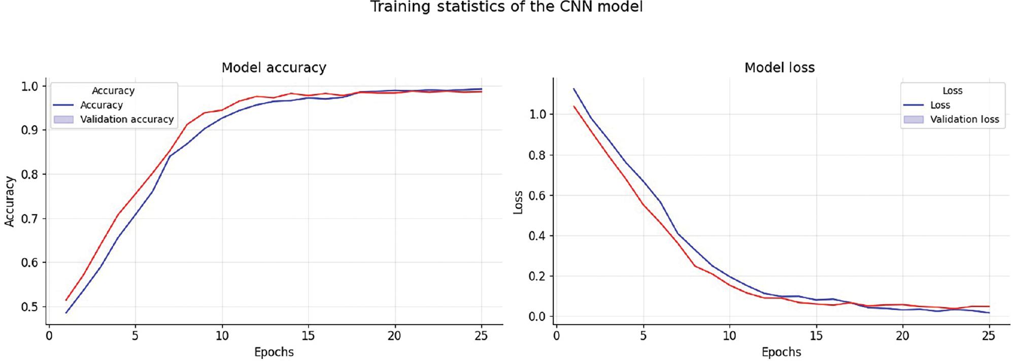
Accuracy and loss throughout the training phase. Abbreviation: CNN, convolutional neural network.
We evaluated the efficiency of the proposed model using multiple well-established measures, such as accuracy and Cohen’s kappa score. Additionally, we created a confusion matrix to assess how effectively the model identifies true-positive, false-positive, true-negative, and false-negative cases across different levels of Alzheimer’s severity.
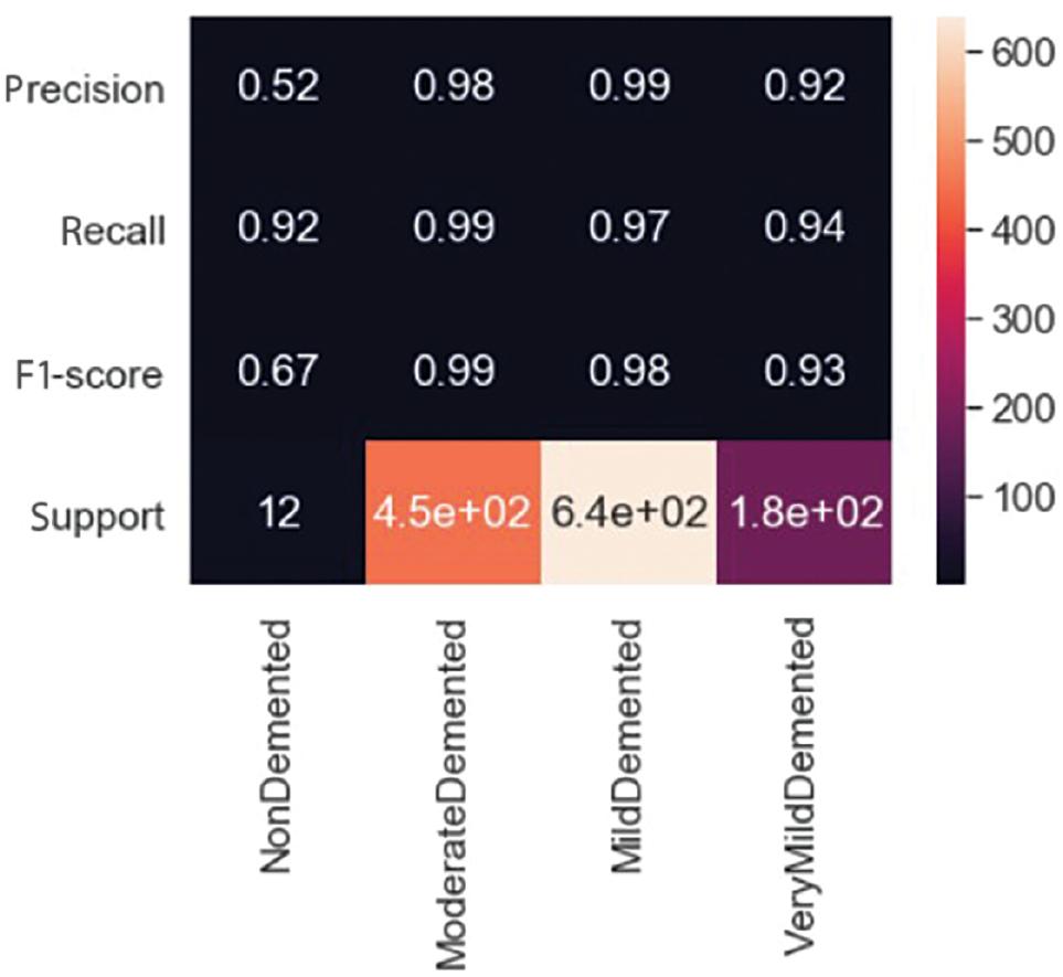
Figure 10 shows the values of the confusion matrix, while Figure 11 displays the ratio of different measures. In the case of “MildDemented,” the confusion matrix indicates that out of the 625 images labeled as “MildDemented,” the model correctly identified 618 of them as “MildDemented.” However, the model has misclassified seven images as “VeryMildDemented.” The F1-score, recall, and precision for the “MildDemented” classification are 0.98, 0.97, and 0.99, respectively.
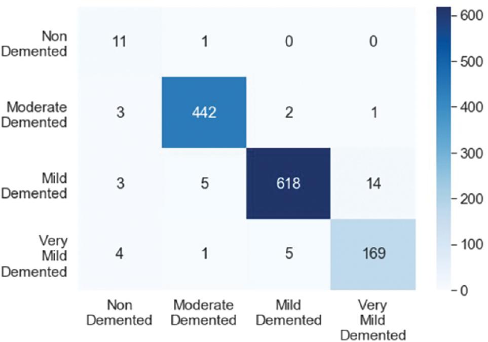
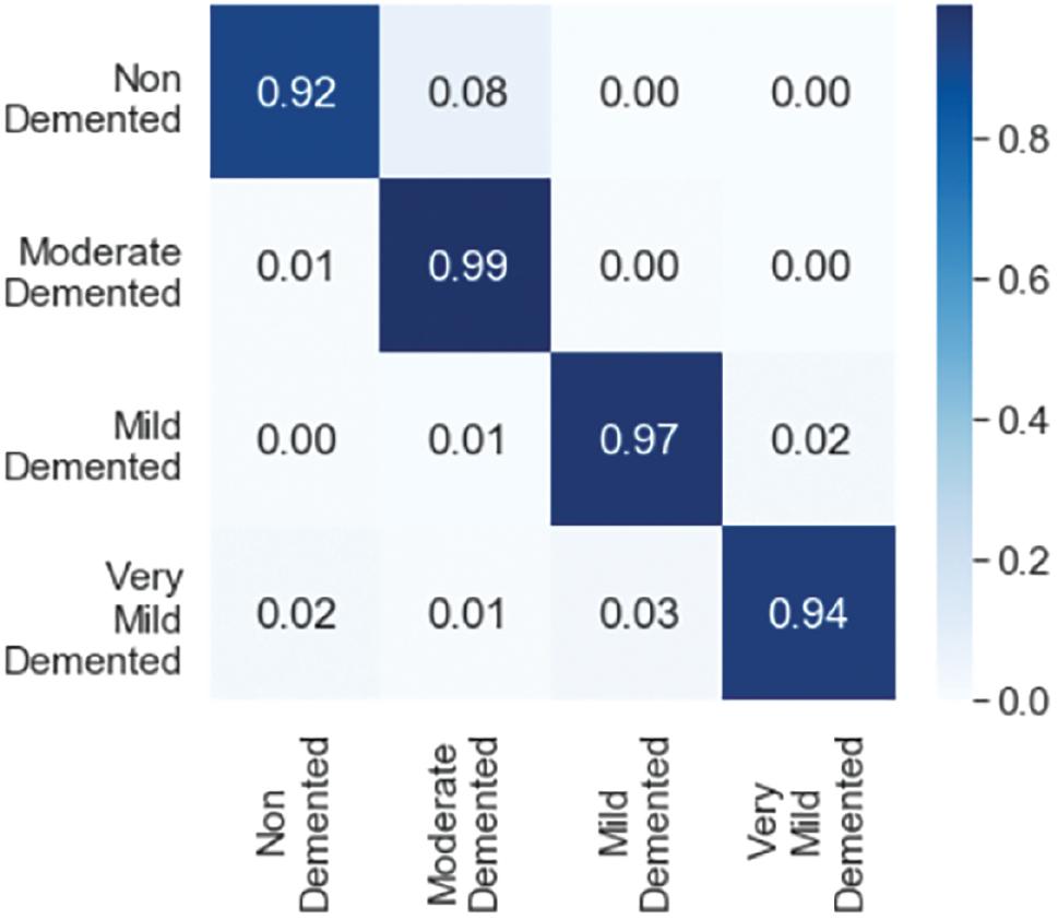
Figure 12 displays the values for each class. It indicates that the model has correctly identified different types of MRI images with 97% accuracy and a Cohen’s kappa score of 0.931. Cohen’s kappa measures the level of agreement between two assessors when assessing a model’s consistency. It ranges from 0 to 1, where a score of 0 indicates chance agreement, while a score of 1 indicates complete agreement. The model employs two strategies, cross-validation and image augmentation, to address the issue of overfitting when the dataset size is limited. However, as we used a substantial dataset, we did not need any specific solution for the overfitting problem.
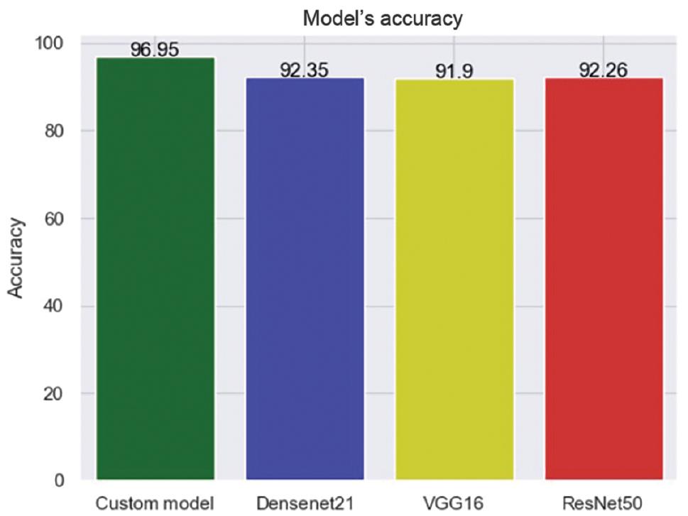
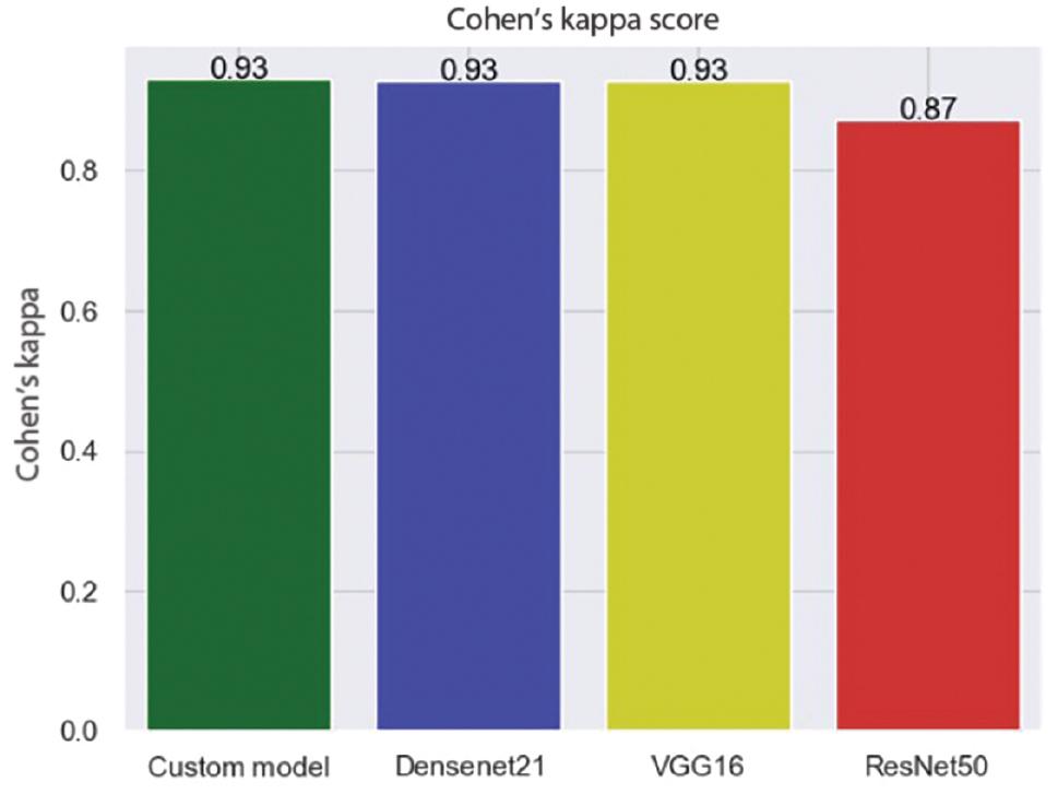
Various pre-trained models, including VGG16, ResNet50, and Densenet21, have been suggested in recent years. These models are used to compare the performance of newly proposed models. To evaluate a proposed model’s performance, it is usually compared with these three models. Therefore, we also examined the performance of these three models.
Among all the models, Densenet21 demonstrated the highest accuracy rate, measuring at 92.35%. Additionally, it received a Cohen’s kappa score of 0.93, indicating excellent agreement between the predicted and actual values. Other models produced unsatisfactory results in terms of accuracy and Cohen’s kappa scores. The comparison outcomes are illustrated in Figures 13 and 14.
CONCLUSION
This study utilized a CNN to classify individuals with Alzheimer’s based on MRI images, addressing data imbalance with a weighted loss function. The proposed model’s performance has been evaluated using well-established metrics, including accuracy and Cohen’s kappa score. The model has achieved an impressive accuracy of 97% and a Cohen’s kappa score of 0.93 on the test dataset. Furthermore, a comparison has been conducted with pre-trained models, such as VGG16, ResNet50, and Densenet21, based on precision and Cohen’s kappa score. The proposed model has outperformed all other models. In the future, we plan to explore alternative methods for feature extraction and conduct a thorough analysis of the model’s behavior. We will also prioritize hyperparameter tweaking to improve the accuracy further. Additionally, we aim to test the effectiveness of the proposed technique by evaluating the models on other available datasets.